Multi-channel integration

Sometimes, a good mapping that maps out all features of an integrand may be hard to find. In this case, we can use multi-channel integration, where different channels focus on different parts of the integrand. This also enables us to incorporate prior knownledge about our integrand.

Toy multi-channel integrand

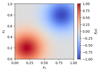
As a toy example, we will look at a two-dimensional function with a positive and a negative Gaussian peak,

\[f(x) = \exp\left(-\frac{\sum_{i=1,2}\left(x_i - \frac{1}{2} + d\right)^2}{2\sigma^2}\right) - \exp\left(-\frac{\sum_{i=1,2}\left(x_i - \frac{1}{2} - d\right)^2}{2\sigma^2}\right)\]

with \(d = 0.3\) and \(\sigma = 0.2\). The integral of this function over \([0,1]^2\) is 0.

Toy integrand for multi-channel integration

MadNIS splits up the integrand into channels by multiplying it with a channel weight \(\alpha_i(x)\) that is normalized over all channels

\[\sum_i \alpha_i(x) = 1 \; .\]

An individual normalizing flow is trained for each of the channels. The channel weights are also computed using a neural network that is trained simultaneously with the flows.

Multi-channel training can be enabled in MadNIS by constructing the integrand using the Integrand class.

import torch
from madnis.integrator import Integrator, Integrand

def integrand_func(x, channel):
    dist = 0.3
    sigma = 0.2
    return (
        torch.exp(-(x - 0.5 + dist).square().sum(dim=-1) / (2 * sigma**2))
        - torch.exp(-(x - 0.5 - dist).square().sum(dim=-1) / (2 * sigma**2))
    )

integrand = Integrand(integrand_func, input_dim=2, channel_count=2)
integrator = Integrator(integrand)
def callback(status):
    if (status.step + 1) % 200 == 0:
        print(f"Batch {status.step + 1}: loss={status.loss:.5f}")
integrator.train(2000, callback=callback)
result, error = integrator.integral()
print(f"Integration result: {result:.5f} +- {error:.5f}")

We set the number of channels to two and enable the training of the channel weights, but do not specify any other information on how to construct the channels. Hence, both start out with a flat mapping and the channel weights are constant over the whole integration domain. The training is then performed as in the single-channel case. The output is

Batch 200: loss=1.00819
Batch 400: loss=0.06211
Batch 600: loss=0.02013
Batch 800: loss=0.01269
Batch 1000: loss=0.02129
Batch 1200: loss=0.00203
Batch 1400: loss=0.00886
Batch 1600: loss=0.01239
Batch 1800: loss=0.01142
Batch 2000: loss=0.00934
Integration result: -0.00028 +- 0.00024

We can see that we get the correct result within the integration uncertainty. To better understand what the networks have learned, we can plot histograms over the generated samples in each of the two channels and the learned channel weights.

import matplotlib.pyplot as plt
samples = integrator.sample(100000)
mask = samples.channels == 0

plt.hist2d(samples.x[mask,0], samples.x[mask,1], bins=30)
plt.show()

plt.hist2d(samples.x[~mask,0], samples.x[~mask,1], bins=30)
plt.show()

plt.scatter(
    samples.x[:,0], samples.x[:,1], c=samples.alphas[:,0], marker=".", vmin=0, vmax=1
)
plt.xlim(0,1)
plt.ylim(0,1)
plt.colorbar()
plt.show()

We can see that each channel only focuses on a single peak of the distribution and the channel weights split the integration domain into two parts.

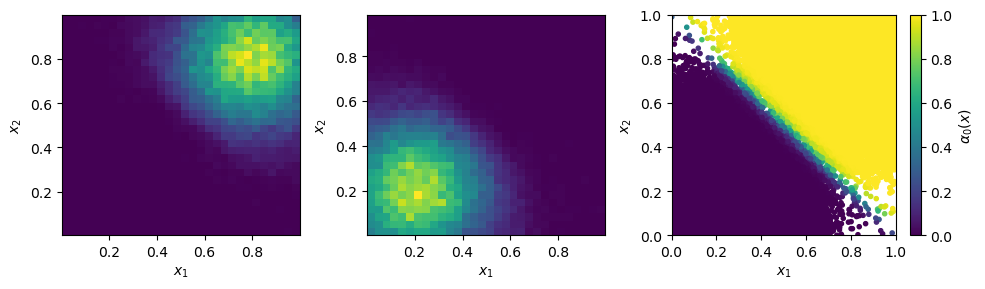
Histograms of the two different learned channel mappings and learned channel weights.

Adding mappings and prior channel weights

While for simple toy examples, MadNIS is able to find sensible decompositions of the integration space into channels, this is usually not easily possible for more complex and high-dimensional integrands. In these cases, prior knowledge about the integrand has to be used to construct the channel mappings and weights. In our toy example, we can construct two mappings such that each one maps more points in one half of the integration space,

\[y = \text{sigmoid}\left(\text{logit}(x) \pm \frac{1}{2}\right) \; .\]

This mapping is invertible and its Jacobian is given by

\[\frac{\partial y}{\partial x} = \frac{y(1-y)}{x(1-x)} \; .\]

The following figure visualizes the resulting probability distributions.

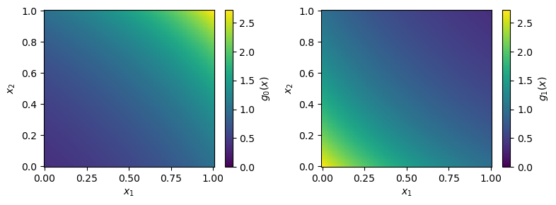
Probability distributions for the analytic channel mappings.

Furthermore, we can specify channel weights that are used as a starting point instead of the uniform initialization from the previous example. One way to define such channel weights is to define them as the probability distribution given by the different channel mappings and normalized in each point. Another way is to define them using parts of the integrand itself. We can rewrite our integrand as

\[f(x) = f_0(x) - f_1(x) \quad\text{with}\quad f_{0,1}(x) = \exp\left(-\frac{\sum_{i=1,2}\left(x_i - \frac{1}{2} \pm d\right)^2}{2\sigma^2}\right)\]

and then use this to define the channel weights as

\[\alpha_{0,1} = \frac{f_i(x)}{f_0(x) + f_1(x)} \; .\]

These mappings and channel weights have to be computed as part of the call to the integrand. Again, this can be done using the Integrand class.

def integrand_func(x, channel):
    y = torch.sigmoid(torch.logit(x) + channel[:,None] - 0.5)
    jac = torch.prod(y*(1-y) / (x * (1-x)), dim=-1)
    dist = 0.3
    sigma = 0.2
    f_0 = torch.exp(-(y - 0.5 + dist).square().sum(dim=-1) / (2 * sigma**2))
    f_1 = torch.exp(-(y - 0.5 - dist).square().sum(dim=-1) / (2 * sigma**2))
    f = f_0 - f_1
    alpha = torch.stack([f_0, f_1], dim=-1) / (f_0 + f_1)[:, None]
    return f * jac, y, alpha

integrand = Integrand(
    integrand_func,
    input_dim=2,
    channel_count=2,
    remapped_dim=2,
    has_channel_weight_prior=True,
)
integrator = Integrator(integrand)

def callback(status):
    if (status.step + 1) % 100 == 0:
        print(f"Batch {status.step + 1}: loss={status.loss:.5f}")
integrator.train(2000, callback=callback)
result, error = integrator.integral()
print(f"Integration result: {result:.5f} +- {error:.5f}")

The dimension of the remapped points \(y\) could be larger than that of the integration space. Therefore, we have to specify their dimension using the remapped_dim parameter. In addition, we set the parameter has_channel_weight_prior to True. The second input to integrand_func contains the index of the channels that each sample is in. The function returns the integrand value multiplied with the Jacobian from the mapping, the remapped point and the channel weights. After the training, we can again take a look at the learned channel mappings and weights using the plotting code from above. (Note that this time we have to plot samples.y instead of samples.x to access the remapped points.)

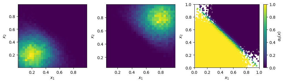
Histograms of the two different learned channel mappings and learned channel weights for a training with analytical channel mappings and prior channel weights.

Like before, every channel has learned to map out one peak of the integrands and the channel weights nicely separate the integration space into two halves. Note that if good prior weights are provided, it might be sufficient to just train the normalizing flows and disable the channel weight training by setting the train_channel_weights option to False, but even then, training the channel weights often leads to further improvements.

Symmetries between channels

Sometimes our integrand has symmetries that we want to make use of. In the example above, we have

\[f(1 - x) = -f(x) \; ,\]

or in other words, the two peaks have the same shape and only differ in their sign. Therefore, the channel mappings used to map out these peaks can be shared between the two channels that we construct. At the same time, every channel still needs its own channel weight. In MadNIS, this can be achieved using the ChannelGrouping class. We have to slightly modify the implementation of the channel mappings compared to the code above such that we can turn one channel into the other with the simple transformation \(y \to 1 - y\).

from madnis.integrator import ChannelGrouping

def integrand_func(x, channel):
    y_0 = torch.sigmoid(torch.logit(x) - 0.5)
    y = torch.where(channel[:,None] == 1, 1 - y_0, y_0)
    jac = torch.prod(y*(1-y) / (x * (1-x)), dim=-1)
    dist = 0.3
    sigma = 0.2
    f_0 = torch.exp(-(y - 0.5 + dist).square().sum(dim=-1) / (2 * sigma**2))
    f_1 = torch.exp(-(y - 0.5 - dist).square().sum(dim=-1) / (2 * sigma**2))
    f = f_0 - f_1
    alpha = torch.stack([f_0, f_1], dim=-1) / (f_0 + f_1)[:, None]
    return f * jac, y, alpha

integrand = Integrand(
    integrand_func,
    input_dim=2,
    channel_count=2,
    remapped_dim=2,
    has_channel_weight_prior=True,
    channel_grouping=ChannelGrouping([None, 0]),
)
integrator = Integrator(integrand)

The training code does not change. The arguments [None, 0] to the ChannelGrouping constructor mean that a regular channel is constructed at index 0 whereas the channel at index 1 reuses the learned mapping of the channel at index 0. Overall, the behavior of the training is similar to that of the previous training without the symmetry. The network again learns a sharped boundary between the two channels in the middle of the integration space. However this time, only a single normalizing flow has to be optimized.

Additionally, the constructor of the Integrator class also has an argument group_channels_in_loss. This also groups channels in the computation of the stratified variance loss, resulting in better numerical stability for trainings with a large number of channels. However, it also prevents the optimization of the relative channels weights within a group of channels.

Stratified training

By default, the training samples are distributed uniformly among the channels during the training. If stratified training is enabled, more samples are generated for channels with higher variance. This allows the training to focus on the most important channels. It can be enabled using the uniform_channel_ratio argument of the Integrator class. It specifies the ratio of samples that are distributed uniformly among channels. The rest is distributed proportional to the standard deviation of the channel (stratified sampling). Setting this parameter to zero can lead to unstable trainings. Values like 0.1 tend to work well in most situations. The training always starts with a warmup phase (depending on the integration_history_length) where the channel is sampled uniformly.

Channel dropping

For trainings with many channels, we often observe that MadNIS reduces the contribution of some channels such that it is close to zero. In this case, it can be useful to disable these channels entirely. To this end, the Integrator class has the options channel_dropping_threshold and channel_dropping_interval. The latter specifies the number of training iterations between checks for channels that can be dropped. The former is a number between 0 and 1. All channels with a combined relative contribution to the total integral that is below this threshold are dropped. If a callback function is used to monitor the training progress, the number of channels that were dropped after a training iteration can be found in the dropped_channels field of the TrainingStatus object passed to the callback function.

Limiting memory usage of buffered training

For buffered training, MadNIS has to store the prior channel weights returned by the integrand. In cases with very many channels, this can require a lot of memory. Since in such cases, the contribution of most channels at a given point will be close to 0, the memory usage can be reduced by only buffering the channel weights of channels with large contributions. The parameter max_stored_channel_weights of the Integrator class specifies the number of stored channel weights. Note that if this option is enabled, both the weights and indices of the channels have to be stored, so the amount of memory used is 2 * buffer_capacity * max_stored_channel_weights * 8 in double precision mode.