Using the MadNIS flow library

In addition to neural importance sampling, the normalizing flow implementation in the MadNIS package can also be used for other applications. The following examples illustrate how unconditional and conditional MadNIS flows can be trained on a toy training dataset.

Simple flow training

As an example distribution, we will look at a two-dimensional Gaussian mixture model with two peaks at \((-1,-1)\) and \((1,1)\) and standard deviations 1 and 0.5. We can generate our training dataset with the code

import torch
data = torch.cat((
    torch.randn((25000, 2)) - 1, 0.5 * torch.randn((25000, 2)) + 1
), dim=0)

Now we can build the MadNIS flow and train it on the data. In this case we will use a Gaussian latent space. Another option would be a uniform latent space, in which case the distribution would be restricted to the unit hypercube. As a loss function, we use the negative log-likelihood.

from madnis.nn import Flow
from torch.utils.data import TensorDataset, DataLoader

loader = DataLoader(TensorDataset(data), batch_size=1000, shuffle=True)
flow = Flow(dims_in=2, uniform_latent=False)
optimizer = torch.optim.Adam(flow.parameters(), lr=3e-4)

for epoch in range(20):
    epoch_losses = []
    for x, in loader:
        optimizer.zero_grad()
        loss = -flow.log_prob(x).mean()
        loss.backward()
        optimizer.step()
        epoch_losses.append(loss.item())
    print(f"Epoch {epoch+1}: loss={sum(epoch_losses) / len(loader)}")

In the last step, we can draw samples from our learned distribution and confirm that the normalizing flow has indeed learned the distribution of the training data by making histograms.

import matplotlib.pyplot as plt
import numpy as np

with torch.no_grad():
    samples = flow.sample(50000)
bins = np.linspace(-5, 4, 50)
plt.hist(data[:,0], bins=bins, histtype="step", label="training data", density=True)
plt.hist(samples[:,0], bins=bins, histtype="step", label="generated", density=True)
plt.xlabel("$x_1$")
plt.legend()
plt.show()

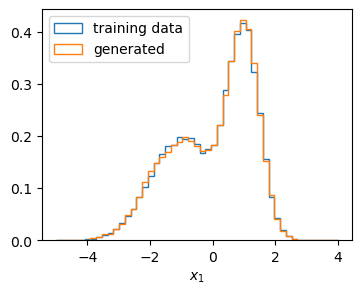
Histogram over samples generated by the trained normalizing flow and its training samples.

Conditional flow training

MadNIS flows can also be used to learn conditional distributions. We again use the Gaussian mixture model from the previous section to obtain points \(x\), but apply a Gaussian smearing with standard deviation 0.5 as a second step, giving us pairs of points \((x, y)\). We can now use conditional flows to, for example, solve the inverse problem, i.e. learn the distribution \(p(x|y)\). This can be done by passing a dims_c argument to the flow constructor and a c argument to the log_prob method.

data_x = torch.cat((
    torch.randn((25000, 2)) - 1, 0.5 * torch.randn((25000, 2)) + 1
), dim=0)
data_y = data_x + 0.5 * torch.randn((50000, 2))

loader = DataLoader(TensorDataset(data_x, data_y), batch_size=1000, shuffle=True)
flow = Flow(dims_in=2, dims_c=2, uniform_latent=False)
optimizer = torch.optim.Adam(flow.parameters(), lr=3e-4)

for epoch in range(30):
    epoch_losses = []
    for x, y in loader:
        optimizer.zero_grad()
        loss = -flow.log_prob(x, c=y).mean()
        loss.backward()
        optimizer.step()
        epoch_losses.append(loss.item())
    print(f"Epoch {epoch+1}: loss={sum(epoch_losses) / len(loader)}")

Once the flow is trained, we can again use it to draw samples and plot histograms. For example, we can check if we recover the distribution \(p(x)\) by sampling from \(p(x|y)\) for \(y \sim p(y)\) and look at the distribution \(p(x|y^{(i)})\) for individual points \(y^{(i)}\).

with torch.no_grad():
    samples_x = flow.sample(c=data_y)
    samples_x0 = flow.sample(c=data_y[0:1,:].expand(10000,2))
    samples_x1 = flow.sample(c=data_y[1:2,:].expand(10000,2))
bins = np.linspace(-5, 4, 50)
plt.hist(samples_x[:,0], bins=bins, histtype="step", label="$p(x)$", density=True)
plt.hist(samples_x0[:,0], bins=bins, histtype="step", label="$p(x|y^{(0)})$", density=True)
plt.hist(samples_x1[:,0], bins=bins, histtype="step", label="$p(x|y^{(1)})$", density=True)
plt.xlabel("$x_1$")
plt.legend()
plt.show()

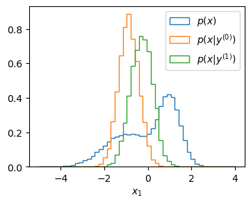
Histogram over samples generated by the trained conditional normalizing flow.

Hyperparameters

There are several hyperparameter that can be passed as arguments to the constructor of the Flow class. The parameters permutations and blocks can be used to control how the coupling blocks are constructed, and which dimensions are transformed conditioned on the other dimensions. The default choice permutaions="log" ensures that every dimension is conditioned on ecery other dimension at least once, and the number of coupling blocks is chosen automatically. Other options include random and exchange. In these cases, the number of coupling blocks has to be specified. For the most fine-grained control, a boolean tensor can be passed using the condition_mask argument to control which dimensions are used as condition for every coupling block.

The arguments layers, units and activaton can be used to change the size of the flow sub-networks. The defaults for the subnet size are relatively small, so making the number of layers and units larger can often lead to improvements. Alternatively, custom sub-networks can be constructed by passing a function to the subnet_constructor argument. The arguments bins, spline_bounds, min_bin_width, min_bin_height and min_bin_derivative determine the hyperparameters of the rational quadratic spline transformation that is the core of the normalizing flows used in MadNIS.

The argument channels can be used to specify the number of channels and build a multi-channel flow, i.e. multiple independent flows that share the same architecture and can therefore be efficiently evaluated in parallel. In this case, the channel argument has to be given when the methods sample, prob, log_prob or transform are called. Lastly, the mapping argument allows to add an additional transformation (or one tranformation per channel in the multi-channel case). For example, this can be used to add preprocessing steps as part of the normalizing flow.