First steps

This tutorial demonstrates how MadNIS can be used to integrate functions. As an example, we will use the function

\[f(x) = \prod_{i=1}^d 2 x_i \; .\]

It’s integral over the unit hypercube \([0,1]^d\) is always \(1\), independent of the number of dimensions \(d\).

Minimal example

Let’s compute the integral in four dimensions. This can be done with the following code

from madnis.integrator import Integrator
integrator = Integrator(lambda x: (2*x).prod(dim=1), dims=4)
integrator.train(100)
result, error = integrator.integral()
print(f"Integration result: {result:.5f} +- {error:.5f}")

We first create an Integrator object with our integrand and its dimension. Then we have to train the integrator for 100 iterations. Lastly, we use combine the information over the integral collected during the training and print the integral and the Monte Carlo integration error in the last line. We get the output:

Integration result: 1.00382 +- 0.00129

Monitoring the training progress

To better monitor the training progress, we can also specify a callback function that is called with a TrainingStatus object after every tenth iteration.

integrator = Integrator(lambda x: (2*x).prod(dim=1), dims=4)
def callback(status):
    if (status.step + 1) % 10 == 0:
        print(f"Batch {status.step + 1}: loss={status.loss:.5f}")
integrator.train(100, callback)
result, error = integrator.integral()
print(f"Integration result: {result:.5f} +- {error:.5f}")

The output is

Batch 10: loss=0.51366
Batch 20: loss=0.23448
Batch 30: loss=0.13336
Batch 40: loss=0.08787
Batch 50: loss=0.05898
Batch 60: loss=0.03766
Batch 70: loss=0.03791
Batch 80: loss=0.02405
Batch 90: loss=0.02370
Batch 100: loss=0.01639
Integration result: 1.00335 +- 0.00127

Computing the integral with more statistics

If we don’t just want to use the samples collected during the training to compute the integral, but draw additional samples using our trained flow, we can also use the integrate function.

result, error = integrator.integrate(1000000)
print(f"Integration result: {result:.5f} +- {error:.5f}")

Here we computed the integral for one million samples. The output is

Integration result: 1.00015 +- 0.00017

Measuring the performance

While the integration error gives us an idea how well the training of the integrator worked, MadNIS offers two functions to get more details. First, we can call the integration_metrics function, again with the number of samples as its argument.

from pprint import pp
pp(integrator.integration_metrics(1000000))

The pretty-printed output is

IntegrationMetrics(integral=0.9999313354492188,
                   count=1000000,
                   error=0.0005457350634969771,
                   rel_error=0.0005457725387231772,
                   rel_stddev=0.17258843067376853,
                   rel_stddev_opt=0.17258842717815095,
                   channel_integrals=[0.9999313354492188],
                   channel_counts=[1000000],
                   channel_errors=[0.0005457350634969771],
                   channel_rel_errors=[0.0005457725492306054],
                   channel_rel_stddevs=[0.17258842289447784])

Most of the fields of the resulting IntegrationMetrics object only become useful for multi-channel integration. One useful quantity for simple single-channel integrals is the relative standard deviation, called rel_stddev, as it measures the integration error independent of the value of the integral and the number of samples. This makes it easier to compare the performance between different integrands with potentially different results.

If the trained integrator is also used as a sampler, another useful set of metrics is returned by the function unweighting_metrics,

pp(integrator.unweighting_metrics(1000000))

Its output is

UnweightingMetrics(cut_eff=1.0,
                   uweff_before_cuts=0.5381982922554016,
                   uweff_before_cuts_partial=0.5381982922554016,
                   uweff_after_cuts=0.5381982922554016,
                   uweff_after_cuts_partial=0.5381982922554016,
                   over_weight_rate=0.0)

From this object, we can read the unweighting efficiency, here around 54%. This tells us which fraction of our (weighted) samples would remain if we applied an accept-reject step based on their weights. In case we have regions in our integration domain where the integrand is zero, the cut efficiency tells us how well our sampler was able to avoid these regions.

Generating samples

After the integrator was trained, we can also use it to generate new samples from the distribution using the sample method. It returns a SampleBatch object containing the sampled points, the corresponding integrand value, the sampling probability and the integration weights. In the following example, we use them to make a histogram of the learned distribution with and without reweighting with the integration weights.

import matplotlib.pyplot as plt
import numpy as np
samples = integrator.sample(1000000)
bins = np.linspace(0, 1, 30)
plt.hist(samples.x[:,0].numpy(), bins, histtype="step", label="learned", density=True)
plt.hist(
    samples.x[:,0].numpy(),
    bins,
    weights=samples.weights.numpy(),
    histtype="step",
    label="reweighted",
    density=True
)
plt.xlabel("$x_1$")
plt.xlim(0, 1)
plt.legend()
plt.show()

This results in the following plot:

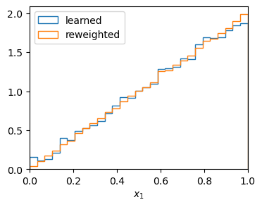
Generated samples with and without reweighting

Buffered training

Often, the function that we integrate is costly to evaluate. In this case, we don’t want to call it in every training iteration and train on a buffer of previously sampled points instead. We can enable it with a few additional arguments to the integrator.

integrator = Integrator(
    lambda x: (2*x).prod(dim=1),
    dims=4,
    buffer_capacity=102400,
    minimum_buffer_size=4096,
    buffered_steps=3,
)
def callback(status):
    if (status.step + 1) % 10 == 0:
        print(f"Batch {status.step + 1}: loss={status.loss:.5f}")
integrator.train(100, callback)
result, error = integrator.integral()
print(integrator.integration_metrics(1000000).rel_stddev)

We set the buffer capacity such that up to 102400 points are buffered. minimum_buffer_size sets the minimum amount of samples in the buffer necessary to start training on them. With the default batch size of 1024, this means that the buffered training starts after the first four batches in our example. buffered_steps specifies how many optimization steps on buffered samples are performed after every training step on fresh samples.

Batch 10: loss=0.49007
Batch 20: loss=0.21208
Batch 30: loss=0.12356
Batch 40: loss=0.07930
Batch 50: loss=0.08147
Batch 60: loss=0.01724
Batch 70: loss=0.01760
Batch 80: loss=-0.00047
Batch 90: loss=0.00252
Batch 100: loss=0.01507
0.17969668280327986

We printed the relative standard-deviation to compare the performance with the previous results. As you can see, they are similar, even though we have reduced the number of calls to our integrand function by a factor of four.